How to move / copy excel sheet from one workbook to another workbook Step by step demonstration

1. Open two Excel workbooks at a time

 

2.    Press "Alt+h+o+m "  

 

This will give following window.

 

 

3.   Press "Alt+t"    (Press both keys simultaneously.  

 Following window will appear.

 4.    Select destination workbook, i.e select the workbook where you want to move sheet. In our example it is Book2, so we have selected book2 in the figure shown above.

5.   Press "Alt+b"  (for placement of sheet )    This step is optional

 

 6.        Press enter key.

it's done.  

 

 

 To  copy excel sheet from one workbook to another workbook

7. After step 2 press "Alt+c "(It will copy the sheet instead of moving .

 

 

 

 

 

 

 

Trace dependent cells in excel / Tracking the value in Excel from trial balance to Balance sheet

Trace  dependent cells in excel

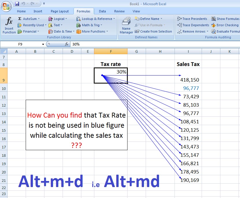
This short cut key is helpful at the time of identifying the value from trial balance which is not going or going many times to balance sheet and due to which balance sheet is OUT.

Step 1 for Trace dependent cells

    Select the value about which we want to find that to which     
        sheet it is going 

Step 2 for Trace dependent cells

      Press the followings keys

         Short Cut key=   Alt+m+d

This will show the green line on the sheet indicating the path of active cell.

In this image small BOX in the green circle indicates that this value of 1,088,384 is going tho other sheet

Step 3 for Trace dependent cells

  "Double Click" on this box it will show the GOTO window ,In 
      above image this is  showing the name of destination of sheet.

Step 4 for Trace dependent cells

   "Double Click" the link in the GOTO window , you will reach Sheet 
      where this value of trial balance is going..

Its done........

 

Auto adjust the height or Word Wrap

1. Normally when we paste the values in the excel sheet the rows

1.1    heights are increased ; or 

as shown below

1.2        complete sentense is not shown in the cell

 as shown below

Reasons:  
2.   Either formatting of cell is 

2.1 set as " word wrap"

2.2 Not "Left alligned"

3. Solution for automatically adjust the height of all cell

3.1 first "Allign the left side " 
( "Alt+H+A+L" i.e Press "Alt" then "h" then "a" then "l")

 

         3.2 then if there is word wrap then cancel it by clicking the                     wrap icon

                                 ("Alt+H+W" i.e Press "Alt" then "h" then  "w")

                        Its done as below

Summary

1.   Alt+H+A+L" i.e Press "Alt" then "h" then "a" then "l")

2. ("Alt+H+W" i.e Press "Alt" then "h" then  "w")

INDEX MATCH Formula in Excel with Step by step illustrations

INDEX MATCH FORMULA

This function is very useful for that kind of job in which we have to find the things from one table and put in front of values present in other table.

Summarising the complete Post

1.              Write Index formula

then

2.     Replace the Row_no part of INDEX formula with MATCH formula.

Comparison of two Formulas

1. Index match 
2. Vlookup 

Index match and Vlookup both are similar. Using both in practical examples it is observed that  index match is better than Vlookup  formula.

          Because;

1. In the Index match formula lookup value can be from any column whether they are in right side or the left side of column containing our required value.
2. It requires only two columns :

                   a). Column in which Lookup value is present.

                   b). Column from which Resultant value is taken.

 However

1. Vlookup   formula works only from left side to right side of table.
2. It requires a continuous array of table and if table contains many column or some column are hidden then it becomes very difficult to calculate index_no for our formula. 

First method (Index Match formula) 

Let we want that when we write “NP”, The formula give us value “7875” As shown in the following fig.

It can be done by using two formulas

          1.     Index
                   2.       Match

1.    INDEX

Syntax
=INDEX(array, row_num, [column_num])     

1.    array :Range from which we have to select our value.(in our example 3rd column i.e “C5:C12” (No. of employees) is the array because we need 7875 from it.)

2.      row_num : Row Number in which 7875 is present( In above example  NP is on 3rd  row so we write 3 in index formula.)

=INDEX(C5:C12,3)

           It will give us 7875

Important thing in the above formula is 3 i.e 3 is Input for Index formula.

2.    MATCH

Syntax

MATCH(lookup_value, lookup_array, [match_type])

1) lookup_value: The value that we want to match in lookup_array. For example, when we look up someone's number in a telephone book, we are using the person's name as the lookup value, but the telephone number is the value we want. (In the given table abov, lookup value is NP.   
 {lookup_value in Vlookup and indexMatch formulas has same nature.}

2) lookup_array: The range of cells being searched. In the given table above, lookup array is A5:A12

3) [match_type]:zero “0” for exact match. It is recommended.

                

a)    =MATCH("NP",A5:A12,0)  or;
b)   =MATCH(F7,A5:A12,0)

(We have used the reference of the cell in second formula. F7 is the cell reference where NP is written.)

Both (a,b) will give us 3

Summary of both formulas

INDEX MATCH

INDEX(C5:C12,3)

MATCH(F7,A5:A12,0)

Now we will copy the complete match formula and paste in place of 3 in the Index formula.           

It gives us following string.

=INDEX(C5:C12,MATCH(F7,A5:A12,0)

                                        

As discussed earlier important thing in the Index formula is 3. Instead of writing the 3 we have used Match formula in its place this formula gives output 3 , which is used as Input for Index formula.

Summarising the complete Post

1.              Write Index formula

then

2.     Replace the Row_no part of INDEX formula with MATCH formula.

Vlook up Formula in Excel with Step by step illustrations

VLOOK UP

This function is very useful for that kind of job in which we have to find the things from one table and put in front of values present in other table.

Comparison of two Formulas

1. Index match 
2. Vlookup 

                   (As discussed in discussion relating  Index match )

               Index match and Vlookup both are similar in their work .
                 Using both in practical examples it is observed
                           that  Index match is better than Vlookup formula.

                                     

                                              Because;

1. In the Index match formula lookup value can be from any column whether they are in right side or the left side of column containing our required value.
2. It requires only two columns :

                   a). Column in which Lookup value is present.

                   b). Column from which Resultant value is taken.

 However

1. Vlookup formula works only from left side to right side of table.
2. It requires a continuouse array of table and if table contains many column or some column are hidden then it becomes very difficult to calculate index_no for our formula. 

Second method (Vlookup formula) 

Let we have a table having three columns first column contains the company names second column contains abbreviation of  company , and third name contains the total number of employees working in that company.

 

Now we want the excel put automatically the number of  employees if we  write the abbreviation of the company in a blank cell. Or;

We want the excel put automatically the Name of company, if we  write abbreviation of company in a blank cell.

As shown below writing the Abbreviation  "acl" in cell F7, Vlookup formula gave result in cell I7

Syntax

=VLOOKUP(lookup_value, table_array, col_index_num, [range_lookup])

1.    lookup_value : It is the value about which we want the information.(Values in “F” column e.g acl, BATAA)

2.  table_array: It is the table from which we want to extract information. (A5:A12 is table array for our exapmple.)

3.  col_index_num: It represents the Number of column from which we want to extract information (In our example 3^rd column is our required information)

4.    [range_lookup]:  What kind of match we want .i.e for exact match select “False” we have selected “False” )

Write formula in the pattern given below.

                       
                       Its done......

For any query and or formula you can write in comments section.........